Multi-Variant Precision Analysis
Nicholas Mikolajewicz
2020-05-28
Source:vignettes/a04_Multi-Variant Precision Analysis.Rmd
a04_Multi-Variant Precision Analysis.RmdMulti-Variant Precision Analyses
Multi-variant precision (MVP) analysis aims to calculate the inherent variability of an instrument and additional error arising from time- or scanner-dependent drifts in scanner calibration. MVP analysis is commonly referred to as multisite-longitudinal precision or reproducibility analysis and is necessary to perform when conducting a multisite or longitudinal clincial trial involving patient scans over multiple scanners and timepoints.
Data import and prep
Prior to analysis, import data and preprocess as described in the Getting Started Vignette.
# import EFP and QC1 imaging phantom data
df.qc1 <-qc1
df.efp <- efp

# omit water-mimetic resin sections
df.qc1 <- dplyr::filter(df.qc1, section  != 1) # remove water mimic section 1
df.efp <- dplyr::filter(df.efp, section  != 4) # remove water mimic section 4
df.efp$section <- as.numeric(as.character(df.efp$section))
df.qc1$section <- as.numeric(as.character(df.qc1$section))

# combine datasets (ensure replicate sets aren't mixed)
df.qc1$replicateSet <- paste("q", df.qc1$replicateSet, sep = "")
df.efp$replicateSet <- paste("e", df.efp$replicateSet, sep = "")
all.data <- bind_rows(df.qc1, df.efp)


# create Calibration Object
co <- createCalibrationObject(all.data)

# get list of feature subsets to analyze
analyze.these <- analyzeWhich(co,
                              include.parameters = c("Tt.vBMD", "Tb.vBMD"))

# preprocess/filter data
co <- preprocessData(object = co,
                      analyze.which = analyze.these,
                      new.assay.name = "preprocessed.data",
                      which.assay = "input")
MVP Analysis
Run mvpAnalysis to perform MVP analysis and store results in Calibration Object. By specifying which.data = “all”, MVP analysis will be performed on all data in the current Assay, and stratified by calibration (uncalibrated vs. calibrated) status if datasets are available.
co <- mvpAnalysis(co,
                   which.data = "all",
                   verbose = F)


# retrieve stored results (as datatables)
mvp.results <-getResults(object = co,
                                which.results = "mvp",
                                format = 'dt')


# show rms statistics for calibrated data
showTable(mvp.results[["rms.statistics"]])
# retrieve stored results (as data.frame)
mvp.results <-getResults(object = co,
                                which.results = "mvp",
                                format = 'df')
# get rms statistics
mvp.rms <- mvp.results[["rms.statistics"]]
# subset rms statistics
mvp.rms.subset <- mvp.rms[grepl(c("long-t12.multi"), mvp.rms$precision.type),  ]
# show table
showTable(mvp.rms.subset, as.dt = T)
Visualize Results
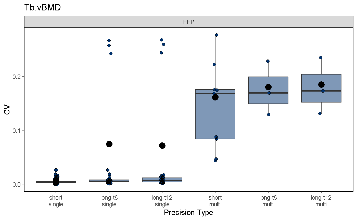
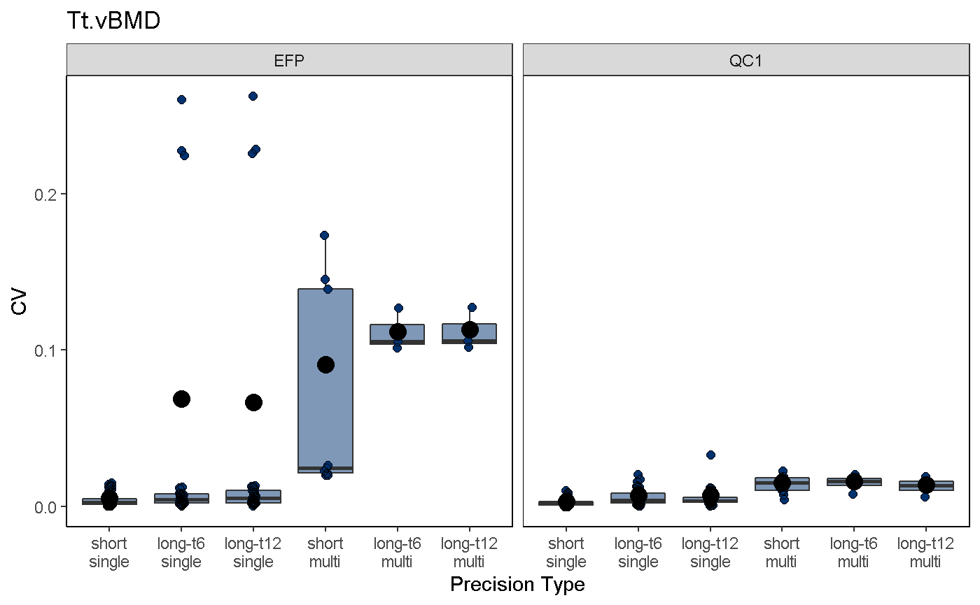
To visualize mvpAnalysis results, use the mvpPlot function. Function arguments are similar to those in the svpPlot function, with the additional option to subselect different precision error types, including:
short: Short-term precision errors only
long: Longitudinal precision errors (i.e., long-term) only
single: Single-site precision errors only
multi: Multi-site precision errors only
all: all of the above (default)
mvpPlot(co,
         outliers = T,
         var2plot = "cv",
         which.data = "all",
         which.precision = "all",
         color.begin = 0.1,
         color.end = 0.5,
         jitter.width = 0.1,
         show.rms.statistic = T)